GRID step
The purpose of the GRID step is to retrieve the systems and staves of the sheet.
Inputs
- The black & white image
- The maximum staff line thickness
- The typical interline value (and the small interline value if any)
Outputs
- The LAG of horizontal sections – See Section and LAG description.
- The LAG of vertical sections
- The staff lines organized in staves
- The global skew of the image
- For every staff:
- the barlines if any
- the vertical connectors if any with a staff above or below
- the starting brace if any
- the starting bracket if any
- The gathering of staves into systems
- The no-staff image
Processing
Filtering runs and sections
First, all the foreground (black) pixels of the binary image are organized into vertical runs.
Then, the engine determines a maximum line thickness, based on the maximum staff line thickness provided by the SCALE step, slightly augmented to cope with potentially thicker ledgers.
Any vertical run which is longer than this maximum staff line thickness cannot be a pure portion of a staff line – it must be a (portion of) crossing object.
Therefore:
- All “long” vertical runs are set aside into the vertical LAG.
- All remaining pixels are organized in horizontal runs gathered in the horizontal LAG.
Then, within each LAG, adjacent runs are organized into sections.
The horizontal sections are further separated between short sections and long sections, because the long sections will drive the staff lines detection.
We can visualize this material. To do so, we have to use the Tools → Constants pull-down menu and there tick the boolean constant displayRuns (it is located in class LinesRetriever).
| Content | View |
|---|---|
| Binary image | 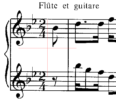 |
| Long vertical sections | 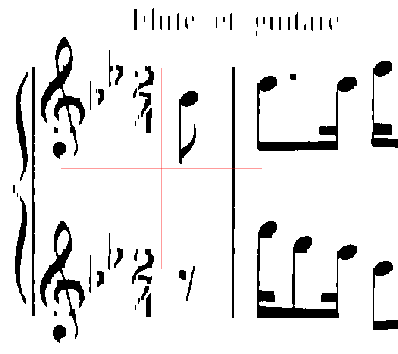 |
| Short horizontal sections | 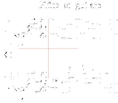 |
| Long horizontal sections | 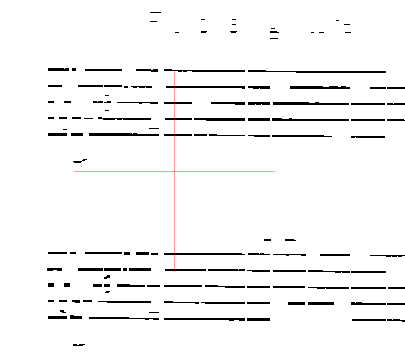 |
Long horizontal filaments
From the set of long horizontal sections, the engine gradually builds long and thin filaments which are likely to correspond to long portions of staff lines.
The filaments that are not straight enough are discarded. A small set of filaments, the longest ones, are used to compute a global slope of the score image. The filaments whose slope diverges from the sheet global slope are discarded.
Then the horizontal filaments are vertically gathered into clusters likely to represent staves. Within a cluster:
- the filaments are expected to be spaced according to a known staff interline
- the number of filaments must match the possible staff sizes (1-line, 4-line, 5-line or 6-line) as defined by the end user via the
Book → Set book parameterspull-down menu.
In the end, the remaining clusters are transformed as standard staves, one-line staves or tablatures according to their line count.
At this point, the left and right abscissa limits of each staff are defined purely via its detected lines.
Staff vertical projection
Since the engine knows the top line and the bottom line for each staff, it can compute a projection of all black pixels located between these two lines onto the x-axis.1
Provided we have activated the PLOTS topic in the pull-down menu, we can visualize this projection:
- either via the
Sheet → Display staves plotspull-down menu - or via the
≡ Staff N°contextual menu from a staff
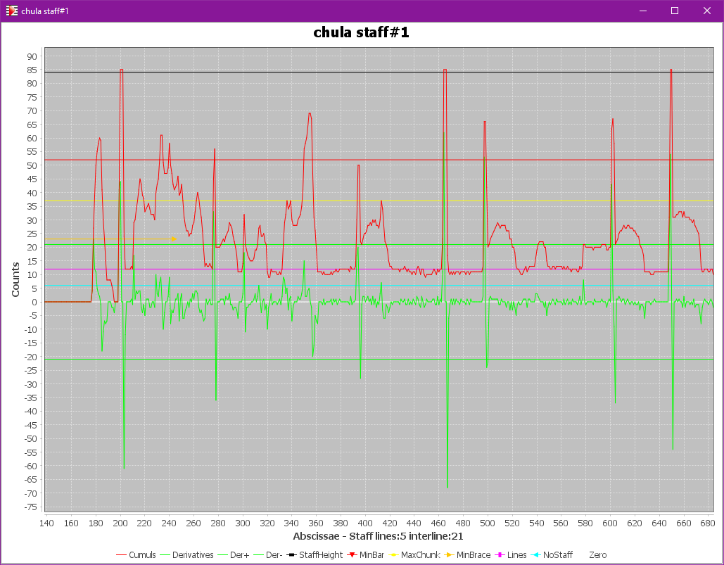
From this projection limited to the staff height, the engine detects peaks which can represent:
- barlines,
- half braces,
- half brackets,
- as well as long stems, etc.
The slim vertical sections located within a peak are used to build vertical filaments. Note that these filaments may extend past the top and/or the bottom of the staff.
If, via the Tools → Constants pull-down menu, we have ticked the boolean constant displayFilaments, then a specific Filaments tab is displayed for both horizontal and vertical filaments initial material:
- The horizontal filaments are in pale red
- The vertical filaments are in pale blue
| Content | View |
|---|---|
| Initial Filaments | 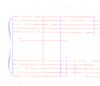 |
All the peaks in vertical projection are handled as vertices in a common peak graph at sheet level. Any vertical alignment detected between a peak in one staff and a peak in the following staff is recorded as an edge in the global peak graph.
Each alignment is then checked for the presence of enough foreground pixels between the two staff peaks, to detect concrete connections between them.
Any filament which extends beyond the staff top or bottom limits and which is not a connector cannot be a barline and is thus discarded.
Based on the detected connections, the engine is now able to gather staves into systems.
System internal alignments
Within each system, the staff peaks are organized into system-based columns.
The starting column, if any, is used to refine the system and staves left abscissa.
The columns found on the right of the starting column must embrace the whole system height, otherwise they are discarded. Also, the peaks that extend past the system vertical limits are discarded.
Brace portions and bracket portions are searched on the left of the starting column. The presence of braces in left margin drives the gathering of staves into parts.
Finally, Inters are created in each system SIG for:
- barlines
- connectors
- braces
- brackets
Results
At the end of this GRID step, we can see the Data tab populated with the grid of systems and staves (shown below in physical and logical modes):
| Mode | View |
|---|---|
 Physical Physical | 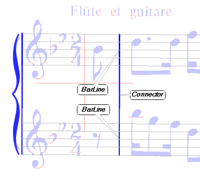 |
 Logical Logical | 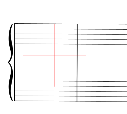 |
Note that some false barlines may persist at the end of the GRID step. They generally get discarded later in the REDUCTION step.
The no-staff image
Since the engine knows which precise horizontal sections compose the staff lines, it can logically “erase” these sections from the binary source and provide what is called the no-staff image.
The no-staff image will be used by several steps down the pipeline.
We can visualize the no-staff image via the Sheet → Display no-staff pull-down menu:
| Content | View |
|---|---|
| No staff |  |
-
In the specific case of a 1-line staff, the engine uses a target barline-height defined as a number of interlines (and perhaps modified via the
Book → Set book parameterspull-down menu). ↩