Pixels assemblies
The BINARY step transforms the input image into a black and white image. From this step on, the image will contain only black (foreground) pixels on a white background.
A (black) pixel is just a black square, of dimension 1 x 1, located at some point (x,y).
Depending on what the engine has to process (staff lines, stems, beams, etc), the same pixels can be viewed through one structure or another.
Run
A horizontal (or vertical) contiguous sequence of pixels of the same color is called a horizontal (or vertical) “run”.
In the same alignment, such run is followed by a run of the opposite color, and so on, until the image border is reached.
A “run table” is a rectangular area, made of sequences of runs, all of the same orientation.
Typically, the whole binarized image can be considered, at the same time, as:
- a table of horizontal runs
- a table of vertical runs
Section
It can be interesting to transitively join adjacent (black) runs of the same orientation, according to some compatibility rules.
Each such resulting assembly is called a “section”.
Typical compatibility rules are:
- Maximum difference in run lengths
- Maximum ratio of difference in run lengths
- Maximum shift on each run end
- Void rule (no check, except adjacency)
Sections are gathered into LAGs (Linear Adjacency Graphs).
Concrete example
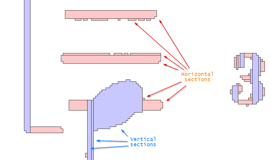
The picture above is displayed, once the GRID step has been performed. We select the “section” view  via the
 View | Switch selections pull-down menu or the F11 function key.
Based on the maximum staff line thickness (previously determined by the SCALE step), this picture combines sections from two different LAG’s:
- From the vertical LAG, all the (vertical) sections with length greater than the maximum line thickness are displayed in pale blue.
- From the horizontal LAG, the remaining pixels are organized in (horizontal) sections and displayed in pale red.